Free for the Digital SAT®
- Reading and Writing and Math practice by domain, skill and difficulty
- Two free full-length tests on official timing: Test A and Challenge Test 1
- The Daily, 1,023 vocabulary words and practice games
Practice until the hard ones feel easy.
Original questions with every answer explained, full-length practice tests and a plan to test day. Pick your test to begin. You can switch any time.
36 free practice questions a day, shared across all your practice, each with a full explanation. No card needed.
free practice questions every day, each with a full explanation
questions in every full-length SAT, in test-day order
SAT vocabulary words to browse, flip and quiz
tests in one place: the SAT, the ACT and AP exams
A quick run with three hearts. String right answers together and the questions get harder while the points multiply.
Every question is tagged by domain and skill, and every answer comes with an explanation.
Practice any single skill at any difficulty, or just the questions you got wrong.
Come back tomorrow and climb. Progress shows your accuracy and your strongest skills.
From a run of the SAT® Daily. Get one wrong and you see exactly why before the next one loads.
If 2x − 7 = 11, what is the value of 3x?
Every full-length SAT® practice test runs in the same order and on the same timing as the digital SAT. The second module of each section adapts to how you did on the first.
The free plan is the real thing, not a trial. When you want everything, pay for the weeks you actually need.
Real daily practice for the SAT, ACT and AP.
$8 × 8 weeks, paid once.
Everything a Test Pass unlocks, two weeks at a time. Good when you don’t have a test date yet.
Prices in US dollars. A Test Pass is $8 for each week until your test, never more than $99 for a test up to 20 weeks away (further out it rises to at most $270), paid once, and ends 3 days after test day. Full refund within 7 days of paying. Under 18? A parent pays: you can send them a payment link.
36 practice questions every day, each with a full explanation, shared across your SAT, ACT and AP practice. The SAT and ACT diagnostics, SAT full-length Test A and Challenge Test 1, ACT Practice Test 1, The Daily and all 1,023 SAT vocabulary words are free too. No card needed.
The digital SAT, the ACT and AP exams. Choose a test at the top of this page. The ACT side has English, Math, Reading and Science practice, lessons, a 20-question diagnostic and full-length practice tests. The AP side has practice by unit and topic and full-length practice exams. Every question is original.
ACT and AP practice use the same free daily questions as SAT practice. The 20-question ACT diagnostic and ACT Practice Test 1 are free too. Other ACT practice tests and the AP practice exams come with a Test Pass or Biweekly.
Every day at midnight Central Time.
No. Peakscor is an independent practice tool, not affiliated with College Board or ACT Education Corp. Scores shown are estimates.
Free, no card. Your first run takes about five minutes.
Take the free SAT diagnosticReach your peak.
A quick run every day, an explanation for every question, and full-length tests on official timing.
Full-length tests
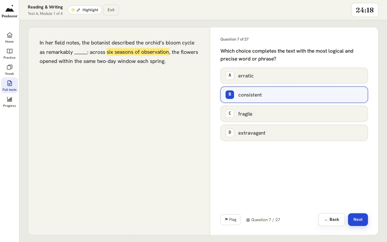
98 questions across four modules, in the same order and on the same timing as the digital SAT, with a highlighter, a question map and a timer you can see.
How it works
A quick run with three hearts. String right answers together and the questions get harder and the points multiply.
Every question is tagged by domain and skill, and every answer comes with an explanation.
Practice any single skill at any difficulty, or just the questions you got wrong.
Come back tomorrow and climb. Progress shows your accuracy and your strongest skills.
Every question is tagged by section, domain, skill and difficulty, so you can practice exactly what you need. Full tests run like test day: two Reading & Writing modules, a break, then two Math modules.
9 easy, 9 medium, 9 hard and 9 challenging questions free every day, each with a full explanation. Filter by section, domain, skill and difficulty. Resets at midnight Central Time.
Take any test on official timing, extended 1.5× time, or untimed to focus purely on accuracy.
Four modules in official order. The second module of each section adapts to how you did on the first.
1,023 essential SAT words. Browse the list, flip flashcards, or quiz yourself.
Accuracy across daily practice and full tests, your strongest skills, and the ones that need the most help.
PEAK Survivor, Peak Hoover and Peak Defense: three games powered by SAT practice questions.
Explanations
Not just the right letter: how to get there, and why the tempting answer is wrong.
A store raises the price of a jacket by 20%. Later, it lowers the new price by 20%. The final price is what percent of the original price?
Check with $100: $100→then$120→then$96
Up 20% means × 1.20. Down 20% means × 0.80.
1.20 × 0.80 = 0.96
The final price is 96% of the original. That’s B.
The 20% cut is taken from the higher price, so it removes more than the 20% increase added.
Test day
Every Peakscor full test follows this order. In the standard tests, the second module of each section adapts to how you did on the first.
27 questions32 min
27 questions32 min
10 min
22 questions35 min
22 questions35 min
98 questions · 2 hr 14 min of testing, plus the break
Plans
The free plan is the real thing, not a trial. A Test Pass unlocks everything until your SAT for one payment. Biweekly does the same, two weeks at a time.
$0no card needed
$18every 2 weeks, cancel anytime
$8a week until your SAT, $99 at most up to 20 weeks away, paid once
Prices in US dollars. Cancel anytime.
FAQ
The Daily, plus 36 practice questions every day: 9 easy, 9 medium, 9 hard and 9 challenging, each with a full explanation. Full-length Test A, Challenge Test 1 and all 1,023 vocabulary words are free too, as are the 20-question diagnostic and PEAK Survivor’s first map. No card needed.
A Test Pass is $8 for each week until your SAT, never more than $99 for a test up to 20 weeks away and never more than $270 for one further out, paid once and never renewed. Biweekly is $18 every 2 weeks and renews until you cancel. Both unlock unlimited practice, every full-length test and Challenge test, the full Learn course, Peak Plan, and every game map and level.
98 questions across four modules, in the same order as the digital SAT: Reading & Writing Module 1 and Module 2 (27 questions each), a 10-minute break, then Math Module 1 and Module 2 (22 questions each). On official timing that’s 2 hr 14 min of testing. You get estimated section scores and a total at the end.
Yes. In the standard full-length tests, Module 2 of each section is the harder version if you get 60% or more of Module 1 right, and the easier version if you don’t. Challenge tests are built from harder material in every module.
Official timing, extended 1.5× time, or untimed, on every test, including the free ones. Extended time allows 48 minutes for each Reading & Writing module and about 52 for each Math module. Untimed removes the clock so you can focus on accuracy.
A quick run with three hearts. Each right answer builds your streak: the questions get harder as it grows, and your points multiply (×2 from three in a row, ×3 from six). A miss costs a heart and drops you back to easy. Best is your longest streak.
Every day at midnight Central Time. You get a fresh 9 easy, 9 medium, 9 hard and 9 challenging.
No. Peakscor is an independent SAT practice tool, not affiliated with the College Board. Scores shown are estimates.
Free, no card.
AP Calculus AB · Unit 7
How to turn a sentence about a rate into a differential equation, and how to check that a function solves one
How a slope field shows the slope at each point, and how to read solution curves from it
How to use a differential equation to find the second derivative and decide concavity
How to solve a separable equation and use an initial condition to find the particular solution
Why a rate proportional to the amount gives exponential growth or decay, and how to use doubling time and half-life
A little under a tenth of the multiple-choice section, roughly 3 to 4 of the 42 questions. That section has a no-calculator part and a part where a graphing calculator is required
The free-response section has 6 questions: 2 in a part where a graphing calculator is required and 4 in a part with no calculator, so practice solving with an initial condition by hand
17 terms. Say what each one means, then open the card to check.
An equation that links an unknown function to one or more of its derivatives. Solving it means finding the function, not a single number.
Example. says the volume of water in a leaking jug shrinks at a rate equal to 0.2 times the volume left.
A function that makes the equation true when you substitute it and its derivative. Check one by differentiating and comparing both sides.
Example. solves for : the left side is and the right side is .
A rate equal to a constant times some quantity. "The rate of change of y is proportional to Q" is written .
Example. If water evaporates from a pond at a rate proportional to its surface area A, then with .
A known value of the solution at one input, such as . It is used to find the constant of integration.
Example. A tank that holds 300 liters when a valve opens gives the initial condition .
Differentiate the right side of with respect to x, using the chain rule on y, then substitute back in. Its sign gives concavity.
Example. For , , so solutions with are concave up.
An object's temperature changes at a rate proportional to the difference between its temperature and the surroundings: with .
Example. A loaf at 82 degrees in a 22-degree kitchen with cools at 3 degrees per minute at first.
A grid of short segments, each drawn with the slope the differential equation gives at that point. It shows the shape of the solutions without solving.
Example. For , the segment at has slope 3 and the segment at is flat.
The graph of one particular solution. In a slope field it runs along the segments, tangent to each one it passes through.
Example. For , the solution curve through is the upper half of the circle .
A constant solution, found where the derivative is zero for every input. In a slope field it shows as a whole row of horizontal segments.
Example. For , the constant function is an equilibrium solution.
Rewrite the equation with every y on the side with dy and every x on the side with dx, then integrate both sides. It works when the right side is a function of x times a function of y.
Example. separates to , so .
The family of all solutions, written with an arbitrary constant such as C. Each value of the constant gives a different curve.
Example. is the general solution of ; and give two of its curves.
The one solution that also meets a given condition, such as passing through a stated point. The condition fixes the constant.
Example. For with , the particular solution is .
The C added after integrating both sides. One C is enough, and it is easiest to find from the initial condition right after integrating.
Example. From and , , so .
When a quantity changes at a rate proportional to itself, , the solution is . It grows if and decays if .
Example. A fictional cell count with and 40 cells at the start follows .
The constant in : the rate of change per unit of the quantity, per unit of time. It is not the factor y is multiplied by each unit of time.
Example. With per year, y is multiplied by each year, not by 1.1.
The time a growing exponential quantity takes to double. From it is , the same from any starting amount.
Example. With per year, the doubling time is years.
The time a decaying exponential quantity takes to fall to half. If with , the half-life is .
Example. A fictional isotope with a half-life of 8 days has per day.
How you’re doing across daily practice and full-length tests.
Your sign-in, plan and preferences, in one place.
Others see your username on leagues, duels and your friends list. You can change it once every 7 days.
To change it we email an 8-digit code to your address first, so only you can do it. Your password is never shown or stored on this device.
Manage billing opens Stripe, where you can change or cancel your plan, update your card and download receipts.
Choose a section, then practice a whole domain or drill a single skill.
Each test mirrors the digital SAT®: 98 questions across four modules, 2 hr 14 min on official timing.
Same 98-question format, built from harder material: a hard Module 1, then a Module 2 made mostly of the hardest questions.
Study the classic SAT® vocabulary list. Browse, flip flashcards, or quiz yourself.
Practice free every day. When you’re ready, get everything until your test for one payment, or pay every 2 weeks.
The Test Pass costs $8 for each week until test day: $99 at most up to 20 weeks away, never more than $270.
$8 for each week until your test, never more than $99 for a test up to 20 weeks away. One payment, and nothing renews.
Everything through 3 days after your test, so you can review it.
$9 a week, billed every 2 weeks. Renews until you cancel. Stop anytime online.
Prices in USD. The Test Pass is one payment and never renews. Biweekly renews every 2 weeks until you cancel, and you can cancel anytime online. Full refund within 7 days of paying. Under 18? A parent pays: you can send them a payment link. Terms
Last updated November 2, 2026 (Do Now live class warm-ups; earlier: Kip is now a study companion with no AI. November 3: College no longer uses AI: feedback, writing help and Essay Writer run in your browser. October 30: College essay drafts and the application checklist, playing a bot in Duels, sharing progress with a parent, Test Pass records, usernames and friends)
Peakscor is an independent SAT®, ACT® and AP® practice website at peakscor.com, built and run by its student founders in Houston, Texas. This policy explains what we collect, why, and what you can do about it. If anything here is unclear, email support@peakscor.com.
Some things are saved only in your browser’s local storage and are never sent to us: the calculator’s layout and saved entries, your practice difficulty and timing, the test you chose last (SAT, ACT or AP), your light or dark theme, your weekly recaps, your best scores on the Daily, today’s practice numbers, this week’s computer rival (made from the average of students at your level), a test in progress, your Test-eve checklist, warm-up answers and how-your-test-went answer, and the questions you’ve seen recently. Your game and study settings, your practice and full-test results, your study plan, your diagnostic result and your mistake notebook are kept in your browser too, and a copy is saved to your guest account or account so they can follow you to another device (see below). You can remove the browser copies by clearing your browser’s site data for peakscor.com.
Your daily free-question count is kept in your browser and on our servers, counted per account and per browser, so the free limit works the same in a private window. The browser is identified only by a scrambled (hashed) version of its random ID, and each count is just a number of questions per difficulty for that day.
So your progress can save, Peakscor creates an anonymous guest account in the background when you visit. It has no name or email address. It is tied to a random ID created when you first visit. It stores:
When you answer a Practice question correctly, finish a lesson, master a module, finish the diagnostic or finish a game, you earn points. We store each award with what earned it (for example a question or lesson ID), the points, the day and the time, plus how long you took to answer, and the league tier you are in. Each week you are placed in a league of up to 30 students at your level. Other students in your league see your display name, your points that week and your rank. They never see your email or anything else about you. Turn on “Hide me from leaderboards” on the Leagues page to stop showing up on any leaderboard right away; you still earn points and see your own total. Points from every test (SAT, ACT and AP) count toward the same weekly league; only you see how your points split by test. Points and league results are kept until you delete your account.
As you study, you earn badges (for example for a 7-day streak, finishing the diagnostic or mastering a unit) and outfits for Kip, the Peakscor mascot. We work them out on our server from what you have already done on Peakscor, and store which badges you earned, when, and which outfit Kip is wearing. Badges and outfits can only be earned, never bought. Only your friends see your badges; other students in a duel with you see Kip’s outfit. They are kept until you delete your account.
With an account you can pick a username (3 to 20 letters, numbers or underscores; please don’t use your real name). It is the name other students see on leagues, duels and boards, and it is how friends find you. You can change it once every 7 days; we store when you last changed it. You can add friends by username or with your own friend link, and you choose whether to accept each request. We store who your friends are, the requests you have sent and received (and whether they came by username or link), the students you blocked, your friend link code and whether you take requests by username. Your friends see your username, Kip in the outfit you wear, your badges, your league (tier, rank and points this week, your best league), your study streak and your duel ratings and record. Nobody else sees your friends list, and a student you block can’t send you requests or open your friend link. Friends, requests and blocks are deleted when you delete your account or remove them.
If you start or join a duel, we store that you are one of its two players (your account ID, never a name or email), its questions, each answer you give (which choice, whether it was right and how long it took), your score and any points it earned you. The other player sees your display name, how many questions you have answered, whether you got each one right once they have answered it too, and your final score. They never see which choice you picked, your email or anything else about you. If you hide yourself from leaderboards, they see “A climber” instead of your name. Anyone you send the link to sees your display name on the invite. Each duel belongs to one test (SAT, ACT or AP), and both players see which. A duel and its answers are deleted 30 days after it ends.
Duel ratings and multiplayer. Rated duels (multiplayer, and friend duels you mark as rated) change your duel rating for that test, which starts at 1000. We store your rating, how many rated duels you won, lost and tied, and your best rating, until you delete your account. Your opponent in a rated duel sees your rating and how much it changed. The Top ratings board shows the 50 highest-rated students’ display names and ratings to everyone signed in; if you hide yourself from leaderboards, you are not on it. Multiplayer matches you with another student: if nobody is free, your duel waits up to a day for the next player, who then plays the same questions.
Playing a bot. If you play a bot in Duels, we store your account ID, which test and bot you picked, the game’s settings and questions, each answer you give (which choice, whether it was right and how long it took) and your score. Nobody else sees it, and it never changes your duel rating or appears on a leaderboard. Which bots you have beaten is kept only on your device.
Timers, leaving a duel and fair play. Each duel question has its own time limit; we store when each question opened, which ones ran out of time, and when your duel page last checked in. If you let 5 questions in a row run out, or your page is gone for 2 minutes during a live duel, you lose that duel. In rated duels only, your duel page also reports, for each question, how long you were away from the duel (in another tab or app), how many times you tried to copy the question, and whether the window was squeezed beside another one. It does not see what you did elsewhere, what other tabs or apps are open, or anything on your screen. A fair-play check combines that with your answer times and right answers to look for outside help (such as a chatbot). If a rated duel is flagged, its rating change is undone for both players. Three flagged rated duels in 14 days pause your rated duels (multiplayer and rated friend duels) for 7 days, then 30 days, then for good; practice, friendly duels and everything else stay open, and the duels page tells you when it ends. If you think a flag was a mistake, email us and a person will review it. We keep the per-question reports with the duel (deleted 30 days after it ends), flags for 180 days, and a pause until 180 days after it ends; all of it is deleted when you delete your account.
Reminders (push notifications), only if you turn them on. When you tap “Turn on reminders” and allow notifications, your browser gives us a push address and two encryption keys for this device. We store them with your account id, your time zone (so we never send before 8 AM or after 9 PM where you are) and the date of the last reminder. We send at most one reminder a day: a duel waiting for your turn, your Summit Sprint day, a streak about to slip, or league news. They never include your name, score or email. Turn them off any time on Home, in Progress or in your account (one tap removes every device); deleting your account deletes them too. Unused for 120 days, they are deleted.
If you join a teacher’s class, we store that you are in the class and the nickname you choose for it. Please don’t use your real name. The teacher sees your nickname and a short summary of your studying: active days in the last week, Learn lessons completed and modules mastered, your diagnostic levels, your practice accuracy by topic, and whether you have finished their assignments. The teacher never sees your email address or your practice answers, and other students never see your data. If you leave the class, or the teacher removes you, the teacher no longer sees any of it. A teacher’s account stores the class name and its join code.
A teacher can run a Do Now: a few questions shown on the classroom screen that students answer on their phones with a 6-digit code, signed in or as a guest. We store that you joined (your account ID or guest account ID, never a name or email) and each answer you give (which choice, whether it was right, and when). The classroom screen shows only how many students picked each answer, never names. Other students never see that you joined or what you answered. On their own class page, the teacher sees how many questions each student got right, by class nickname, only for students who are in that class; anyone else is counted without a name. If you make a free account at the end, your answers stay with it. Do Now records are deleted 30 days after the Do Now.
With an account you can turn on “Share progress with a parent” on your Account page. It makes a private link (peakscor.com/p/…) to a page for a parent or guardian with your weekly progress: minutes practiced, questions answered and accuracy this week and last week, skills you improved, your estimated score range, your streak, your test or exam date and countdown, and whether your plan is paid and until when. If you type a first name or nickname for the page, it shows that; otherwise it says “Your student”. Please don’t use your full name. The page never shows your questions, answers, mistakes, email address or username.
While the link is on, the app sends us those totals (never your answers) so the page stays current. We store the nickname, the totals, a count of how many times the page was opened (no IP address or device details) and a scrambled fingerprint (hash) of the link, never the link itself; your device keeps the link so you can copy it again. We never send the link to anyone: you copy or share it yourself. Anyone who has the link can open the page, so share it only with your parent or guardian. You can make a new link (the old one stops working right away) or turn it off at any time, which deletes everything about it from our servers; deleting your account deletes it too. The page has no ads or trackers, and search engines are told not to list it.
Like any website, our hosting providers process your IP address and basic request details (such as browser type) to deliver pages and keep the service secure. A sign-in token for your guest account or account is kept in your browser’s local storage. When someone makes an account, we keep the email address they signed up with and scrambled (hashed) versions of their IP address and browser ID for up to 31 days, only to stop disposable email addresses and limit how many accounts one network or browser can create. If a page breaks, your browser may send us a short error report: what went wrong, which page it happened on (without anything after the “?” in the address), the site version and your browser type. Email addresses and sign-in tokens are removed from it, and it doesn’t include your user ID or email address. We keep error reports for about 30 days. We don’t use advertising cookies or third-party analytics tools.
We also count visits to our own pages, without identifying anyone. When a page opens, your browser sends our server the page name, a coarse source (a campaign tag in the link, or the website that sent you), a device size class (phone, tablet or desktop), and whether it is your first visit today. The server adds these to day-by-day totals. It does not save your IP address, your account, a cookie or any device ID with them, so a total can’t be traced back to you. We skip this count entirely if your browser sends a Do Not Track or Global Privacy Control signal.
Kip is your built-in Peakscor study companion, helping you find lessons, understand your progress, and discover what to practice next. Kip is not an AI. You can type a question, and Kip answers by matching your words to Peakscor’s own pages and lessons with fixed rules; its suggestions come from simple rules applied to your own practice, lessons and study plan.
Until November 2026, Kip was an AI chat. Messages sent to it went to Anthropic, the company that made the AI model, which handled them as a service provider under its commercial terms: it didn’t use them to train its models and deleted them within 30 days, except that it could keep a message for up to 2 years if its safety systems flagged it, or longer if the law required. Old chats stayed only in your browser, and we still keep, for up to 90 days, the daily counts of those messages, which never included any text. Clearing your browser’s site data for peakscor.com removes old chats from your device.
Kip is a study helper, not a counselor, and nobody at Peakscor is watching what you do with it. If you’re thinking about hurting yourself or you don’t feel safe, call or text 988 (the Suicide & Crisis Lifeline) any time, day or night, and tell a trusted adult, like a parent, school counselor or teacher, right away. If you’re in immediate danger, call 911.
College essays are personal, and many of our students are under 18, so College handles them with extra care. Nobody at Peakscor reads your essays as part of running the site, and we don’t use them for anything except saving them for you.
Your application checklist saves the same way: to your account if you’re logged in, or to that browser if you’re not. We keep which items you ticked and when.
College doesn’t use AI. Feedback, every writing-help tool, the brainstorm tips, the Toolkit helpers and the word counts work in your browser using fixed rules. Your essays, notes and answers are never sent to an AI company or anyone else for this, and the results aren’t saved.
Essay Writer keeps the notes you jot under each paragraph, and the format you picked, in that browser only. They never go into your essay and never reach our servers. They’re removed when you delete that essay or sign out, and clearing your browser data erases them.
Before November 3, 2026, students with an account could ask for AI help, and that text went to Anthropic. If you used it, Anthropic handled the text as described under “Kip’s earlier AI chat” above. We still keep, for up to 90 days, the daily counts of those requests, which never included any text.
If your essay mentions something like self-harm, Feedback shows free, confidential support resources next to it. That check also runs in your browser: nothing about it is recorded or sent to anyone. The same goes for the guidance under “If you’re going through something hard” above.
Only to run Peakscor: to sign you in, save and sync your progress and your essay drafts, grade questions, show leaderboards, keep the service secure and fair, handle payments if you buy a plan, and reply when you contact us. We don’t use your data for advertising, and we don’t use it to train AI models.
We don’t sell or rent personal information. We use a small number of service providers who process data only to run Peakscor:
We may also share information if the law requires it, or to protect the safety of students or the security of the service.
Game leaderboards are public and show your display name and your scores. They never show your email address. If you join a class, its teacher sees the summary described under “Classes”. In a Do Now, the classroom screen shows only how many students picked each answer, never names (see “Do Now”). In a duel, the other player sees what is described under “Duels”. If you turn on “Share progress with a parent”, anyone with that private link sees what is described under “Sharing progress with a parent”. Other students in your weekly league see your display name, points that week and rank, and the Summit Sprint board shows your display name, days climbed and sprint points, unless you turn on “Hide me from leaderboards”. Nothing else about your account is public.
Peakscor is meant for students 13 and older, and we don’t knowingly collect personal information from children under 13. If you believe a child under 13 has made an account, email us and we will delete it.
These choices are available to everyone, wherever you live.
We keep account and guest data until it is deleted. Duels are deleted 30 days after they end, and bot games 30 days after they start. Do Now records (who joined and their answers) are deleted 30 days after the Do Now. Duel fair-play flags are kept for 180 days, and a pause of rated duels until 180 days after it ends. The list of which duel questions you were dealt (so you never get the same one twice) is kept until you delete your account. Kip message counts are kept for 90 days, and your chats with Kip stay on your device until you delete them. When you delete your account, it is erased from our database right away. Copies in our providers’ encrypted backups are overwritten on their normal schedule, usually within a few weeks.
Purchase agreement records are kept for 3 years after a plan ends, even if the account is deleted, because subscription laws require us to be able to show what was agreed to. They are kept apart from the account and used for nothing else.
All traffic is encrypted. Every database table has access rules so that each student can read only their own records, and those rules are tested automatically whenever the code changes. No system is perfectly secure, so if you think something is wrong, tell us right away.
Peakscor is independent. It isn’t provided by or through any school, and we don’t receive student records from schools. A teacher can make a Peakscor class and invite students with a code; joining is up to each student, and the teacher sees only the class summary described under “Classes”.
If we change this policy, we will update the date at the top. If a change affects how we use data you’ve already given us, we will tell you on the site before it takes effect.
Questions or requests: support@peakscor.com.
Last updated October 25, 2026 (Test Pass prices for test dates more than 20 weeks away; earlier: Biweekly replaces Weekly)
These terms cover your use of Peakscor at peakscor.com. By using Peakscor, you agree to them. If you don’t agree, please don’t use the site.
You must be at least 13 years old to use Peakscor or make an account.
Only adults can buy a plan. The person who pays must be 18 or older. If you are under 18, a parent or guardian buys the plan for you: in the upgrade dialog, choose Under 18? Send this to a parent, and they pay on Stripe’s secure page with their own email and card. The person who pays agrees to these terms for themselves and, when the plan is for a student, on the student’s behalf.
Keep your sign-in details private, use your own email address, and don’t share your account. You are responsible for what happens on your account. You can delete it at any time from the account menu.
The free plan is free and needs no card. Paid plans (the Test Pass and Biweekly) unlock more practice, tests and lessons, as described on the Pricing page.
Please don’t:
Peakscor’s questions, explanations, lessons, games and design are our original work and belong to Peakscor. You may use them for your own studying. Teachers and tutors who want to use them with students should email us first. Read how our questions are made.
If you send us feedback or report a problem with a question, we may use it to improve Peakscor without owing you anything.
Peakscor is an independent practice tool. It is not affiliated with, endorsed by or sponsored by the College Board or ACT Education Corp. Our questions are original practice in the style of each test, not official test questions. Scores shown on Peakscor are estimates, and we don’t promise any particular result on the SAT, the ACT or any AP exam.
SAT®, AP® and Advanced Placement® are trademarks registered by the College Board, which is not affiliated with, and does not endorse, Peakscor. PSAT/NMSQT® is a registered trademark of the College Board and the National Merit Scholarship Corporation, which are not affiliated with, and do not endorse, Peakscor. Bluebook™ is a trademark of the College Board. ACT® is a registered trademark of ACT Education Corp., which is not affiliated with, and does not endorse, Peakscor. Common App is a trademark of The Common Application, Inc., which is not affiliated with, and does not endorse, Peakscor. Desmos is a trademark of Desmos Studio PBC.
If you believe something on Peakscor copies your work or misuses your trademark, email support@peakscor.com and tell us what it is and where it appears. We will reply within one business day and take the content down while we review it.
We work hard to make Peakscor accurate and reliable, but it is provided “as is.” Questions or explanations may sometimes contain mistakes, and the site may sometimes be unavailable.
College guides and AI writing help are general guidance. They aren’t an official admissions evaluation, they can contain mistakes, and they can’t predict or promise any admissions decision. Requirements change, so confirm them with each college. What you submit is yours: you’re responsible for making sure it’s accurate, it’s your own work, and it follows the rules of the Common App and of each college you apply to, including their rules about AI.
To the extent the law allows, Peakscor is not liable for indirect or consequential losses, and our total liability for any claim is limited to the amount you paid us in the 12 months before the claim, or $50 if you paid nothing.
You can stop using Peakscor at any time. We may suspend accounts that break these terms. If we ever shut Peakscor down, we will refund the unused part of any paid subscription.
These terms are governed by the laws of the State of Texas.
We may update these terms. We will change the date at the top, and tell you on the site about any important change before it takes effect.
Last updated October 28, 2026
Every question, passage, explanation and lesson on Peakscor is original practice in the style of the test it prepares you for. None of it is an official SAT®, ACT® or AP® question, and we are not affiliated with the College Board or ACT.
Scores on Peakscor are estimates based on how you do on our practice questions. They are not official scores and don’t predict an exact result. ACT scores come from our own model, not from ACT conversion tables.
If a question looks wrong, or you think something is too close to published material, email support@peakscor.com. We reply within one business day and take reported content down while we review it.
Unlimited practice, every full-length test and the full course. Checking checkout…
Save your progress and pick up where you left off.
Your account keeps game coins, characters and map progress in sync across devices. Practice history stays on this device.
By continuing, you agree to the Terms and Privacy Policy and confirm you’re 13 or older.
